
How to Plan a Data Science Project ?

The foundation of any data science project is a thorough understanding of your dataset. I'm gonna mention here some key steps to follow to complete a DS project:
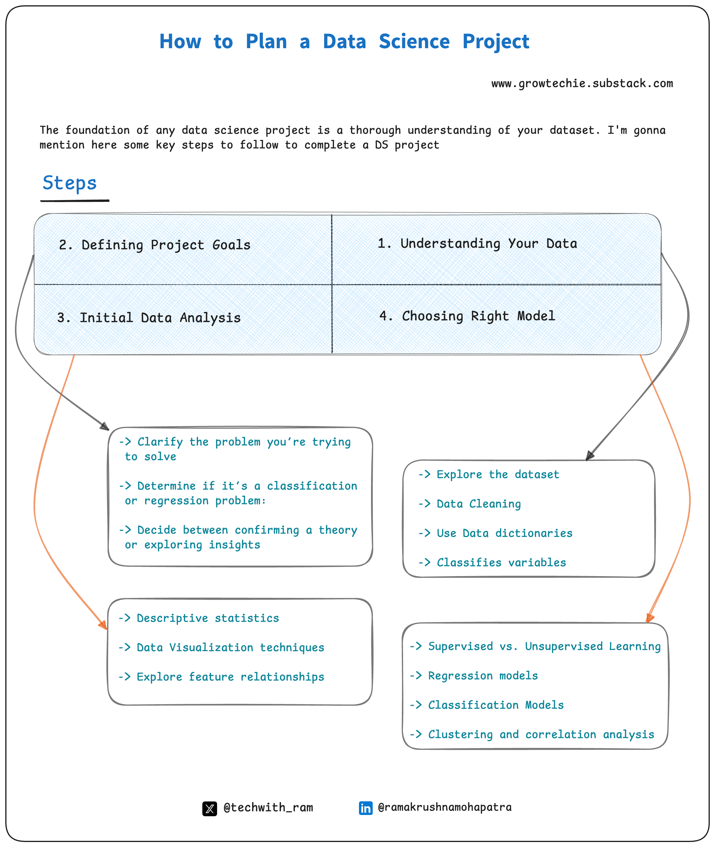
1. Understanding Your Data
A solid grasp of your dataset lays the foundation for a successful project. Here’s how to approach it efficiently:
Explore the Data: Use Python's pandas to get a quick overview:
df.head()→ Preview the first few rowsdf.info()→ Check data types and missing valuesdf.describe()→ Get summary statistics
Handle Missing Values: Identify gaps with df.isnull().sum(). Decide whether to impute (fill in) or remove them, as this impacts model performance.
Use a Data Dictionary: Like a map legend, a data dictionary explains each variable. If unavailable, create one—it improves clarity throughout the project.
Classify Variables: Distinguish categorical (nominal, ordinal) from numerical (interval, ratio) data. This helps guide analysis and model selection.
2. Defining Project Goals
Clear goals shape your entire analysis. Here’s how to define them effectively:
Identify the Problem: Are you predicting house prices (regression) or classifying customer churn (classification)? Defining the objective ensures a focused approach.
Choose the Right Model Type:
Regression → Predict continuous values (e.g., sales forecasts).
Classification → Predict categorical outcomes (e.g., fraud detection).
Set Your Analytical Approach: Are you testing a hypothesis or exploring insights? This choice determines whether you validate a theory or uncover new patterns.
3. Initial Data Analysis
Before building models, explore your data to gain insights and identify key patterns. Here’s how:
Descriptive Statistics: Get a summary of numerical variables.
df.describe()– Provides mean, median, standard deviation, and percentiles.df.mean(),df.median(),df.std()– Compute specific statistics.
Data Visualization: Identify patterns and distributions.
df.hist(bins=30)– Plot histograms for numerical columns.sns.boxplot(x='feature', data=df)– Visualize outliers using a box plot.sns.pairplot(df)– Examine variable relationships with scatter plots.
Feature Relationships: Detect correlations for feature selection.
df.corr()– Compute correlation matrix between variables.sns.heatmap(df.corr(), annot=True, cmap='coolwarm')– Visualize correlations.
4. Choosing the Right Model
Selecting the right model is like choosing the best tool for the job—it depends on your data and project goals. Here’s a structured breakdown:
→ Supervised vs. Unsupervised Learning
✔ Supervised Learning (Labeled Data) – Predict a target variable. Examples:
Regression: Predict continuous values (e.g., house prices).
Classification: Predict categories (e.g., spam detection).
✔ Unsupervised Learning (No Labeled Data) – Discover hidden patterns. Examples:
Clustering: Group similar data points (e.g., customer segmentation).
Dimensionality Reduction: Identify key features (e.g., PCA).
from sklearn.model_selection import train_test_split

X_train, X_test, y_train, y_test = train_test_split(X, y, test_size=0.2, random_state=42)
Regression Models (Predicting Continuous Values)
Linear Regression: Assumes a straight-line relationship.
Polynomial Regression: Captures non-linear trends.
Random Forest Regression: Handles complex relationships well.
Gradient Boosting (XGBoost, LightGBM): Powerful ensemble models.
from sklearn.linear_model import LinearRegression

model = LinearRegression()
model.fit(X_train, y_train)
y_pred = model.predict(X_test)
Classification Models (Predicting Categorical Outcomes)
Logistic Regression: Simple and interpretable for binary classification.
Decision Trees: Rule-based classification.
Support Vector Machines (SVM): Effective for both linear and non-linear classification.
K-Nearest Neighbors (KNN): Classifies based on nearby data points.
Neural Networks: Ideal for complex patterns with large datasets.
from sklearn.linear_model import LogisticRegression

clf = LogisticRegression()
clf.fit(X_train, y_train)
y_pred = clf.predict(X_test)
Clustering & Pattern Discovery
K-Means Clustering: Groups similar data points.
PCA (Principal Component Analysis): Reduces data dimensionality.
Association Rule Learning: Finds relationships between variables.
from sklearn.cluster import KMeans

kmeans = KMeans(n_clusters=3, random_state=42)
kmeans.fit(X)
labels = kmeans.predict(X)
Model Selection Considerations
→ Dataset Size & Quality – More data can enable complex models.
→ Interpretability – Simple models (e.g., linear regression) are easier to explain.
→ Computational Resources – Some models (e.g., deep learning) require high processing power.
→ Performance vs. Complexity Trade-off – Start simple, then iterate.
Planning is the cornerstone of any successful data science project. By thoroughly understanding your data, defining clear objectives, performing initial analysis, and selecting the right modeling approach, you lay a solid foundation for the entire process. Just like preparing for a long journey, meticulous planning ensures a smoother and more efficient path forward.
Every data science project is a unique journey. While these steps provide a strong starting point, flexibility and adaptability are key. With thoughtful planning and a strategic approach, you’ll be well-equipped to navigate challenges and uncover valuable insights hidden within your data.
Follow me on socials:
Twitter: @techwith_ram
Linkedin: @ramakrushnamohapatra
 | A guest post by
|