
Build Your First Neural Network

Most people learn neural networks by calling .fit() and watching accuracy go brrrrr.
That’s fine… until you realize you still don’t really know why anything is happening under the hood. This post is for the people who want to peel the black box open just a little.
We’re going to build a small but real neural network using only NumPy, step by painful-but-satisfying step. No PyTorch, no TensorFlow, no Flax, no Keras, no .backward(), no autograd.
Just matrices, loops, and the chain rule scribbled on paper (or in your head if you’re brave).
By the end you’ll have:
written forward and backward passes yourself
watched a loss number actually drop from “terrible” to “pretty decent”
made a tiny network learn to guess someone’s gender from height & weight (classic toy example)
understood why people scream about vanishing gradients, why sigmoid kind of sucks sometimes, and why backprop feels like reverse-engineering your own mistakes
If you already know:
what a dot product is
roughly how sigmoid squashes numbers between 0 and 1
that training = repeatedly nudging weights to make predictions less wrong
…then you’re more than ready.
Even if some parts feel shaky, that’s okay. We’ll go slowly, look at shapes a lot, and print stuff to see what’s moving. Let’s open a notebook, and let’s build something that learns from scratch, together. Ready when you are.
Let’s start with one lonely, confused neuron…
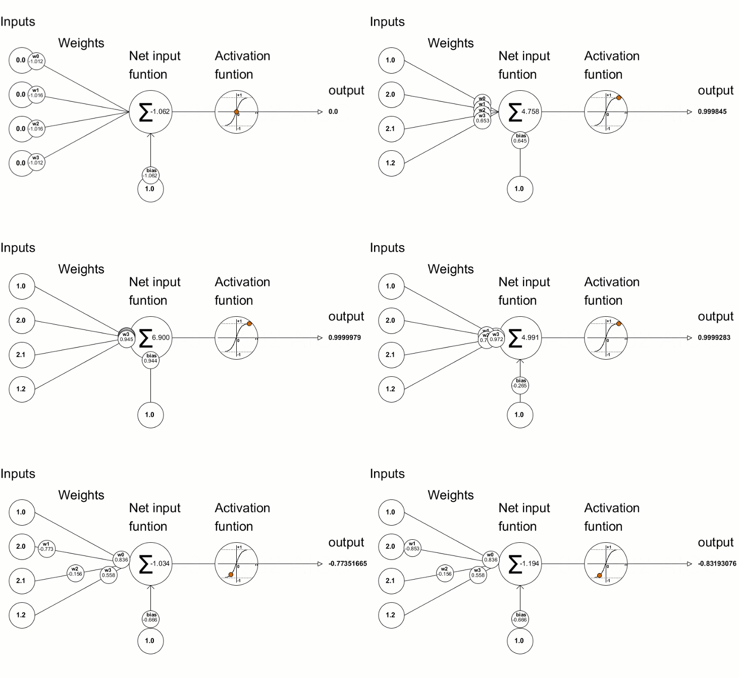
1. One lonely neuron first: A single artificial neuron does two things:
a. weighted sum + bias
b. activation function
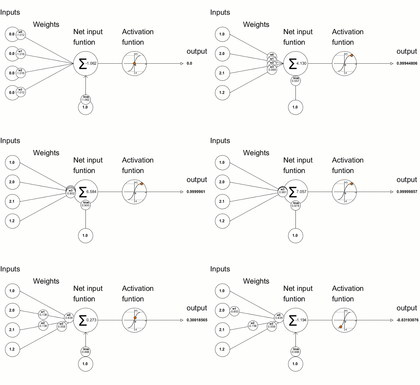
Source: Here. [Single Neuron]
import numpy as np

def sigmoid(z):
    return 1 / (1 + np.exp(-z))

# Example: one input, one weight, one bias
x = 0.8
w = 1.5
b = -0.9
z = w * x + b           # linear part
y = sigmoid(z)
print(f”Output: {y:.4f}”)   # something between 0 and 1
Now the same thing, but cleaner as a class.
class SingleNeuron:
    def __init__(self, w, b):
        self.w = w
        self.b = b

    def forward(self, x):
        z = np.dot(self.w, x) + self.b
        return sigmoid(z)

# Multiple inputs now
w = np.array([0.4, -1.2, 0.7])
b = 0.1
neuron = SingleNeuron(w, b)
x = np.array([1.0, 2.0, -0.5])
print(neuron.forward(x))
That’s feedforward for one neuron. Easy.
So, what’s happening here?
Imagine you’re a very simple brain cell (a neuron) sitting inside a network. Your job is to look at several pieces of information coming toward you (in this case 3 numbers: 1.0, 2.0, and -0.5) and then decide how strongly you want to “fire” (send a signal forward). But you don’t treat all incoming signals equally.
Some kinds of information excite you → you give them positive weight (like 0.4 or 0.7)
Some kinds of information annoy/upset/inhibit you → you give them negative weight (like -1.2)
You get some numbers as input → x = [1.0, 2.0, -0.5]
Each has its own importance (weight) → w = [0.4, -1.2, 0.7]
You do:
(0.4 × 1.0) + (-1.2 × 2.0) + (0.7 × -0.5) = -2.35
Add your personal offset (bias) → -2.35 + 0.1 = -2.25
Then squash it with sigmoid → turns -2.25 into ≈ 0.095
So the neuron says, “I’m only ~9.5% activated right now.” That’s it.
Everything big (ChatGPT, Gemini & image models…) is just tons of these little guys connected together doing exactly this. The class just keeps the neuron’s “personality” (weights + bias) in one place and gives it a clean forward() button.
2. Let’s stack layers—a proper (tiny) network.
Most tutorials jump straight to training. I think it’s worth seeing the shapes first without training pressure.
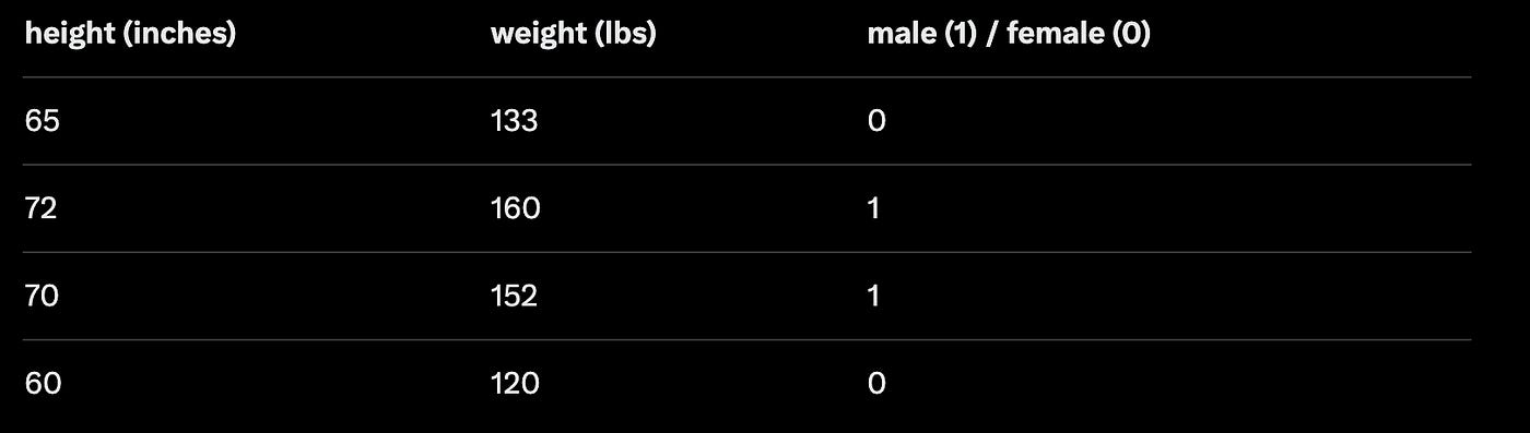
Task: height + weight → probability (person is male)
Dataset (classic toy example):
# Let’s center roughly around median-ish values
X = np.array([
    [65-67, 133-140],   # roughly centered
    [72-67, 160-140],
    [70-67, 152-140],
    [60-67, 120-140]
])   # shape: (4, 2)

y = np.array([[0], [1], [1], [0]])   # (4, 1)
Network layout:
Input: 2 features
Hidden layer: 4 neurons (small but enough to learn something non-linear)
Output: 1 neuron → sigmoid → probability
np.random.seed(42)

# Layer 1 (input → hidden)
W1 = np.random.randn(2, 4) * 0.3    # smaller init → stabler start
b1 = np.zeros((1, 4))

# Layer 2 (hidden → output)
W2 = np.random.randn(4, 1) * 0.3
b2 = np.zeros((1, 1))

# Forward pass (one time - no training yet)
z1 = X @ W1 + b1
a1 = sigmoid(z1)           # (4,4)
z2 = a1 @ W2 + b2
y_hat = sigmoid(z2)        # (4,1)

print(”Random network predictions (terrible):”)
print(y_hat.flatten().round(3))
You’ll see numbers all over the place; that’s expected.
3. The only thing that matters: how wrong are we?
We’ll use binary cross-entropy (most natural for 0/1 classification)
def bce_loss(y_true, y_pred):
    # tiny epsilon prevents log(0)
    eps = 1e-8
    return -np.mean( y_true * np.log(y_pred + eps) +
                    (1 - y_true) * np.log(1 - y_pred + eps) )
4. Backpropagation—the heart of the whole thing
This is where most people get scared. The truth is it’s just the chain rule applied many times.
We want four things:
∂L/∂W2
∂L/∂b2
∂L/∂W1
∂L/∂b1
Luckily when you use sigmoid + BCE together, the math simplifies beautifully at the output layer:
# -----------------------
#        BACKPROP
# -----------------------

# Output layer gradients
dz2 = y_hat - y                        # (4,1)   ← magic simplification!
dW2 = (a1.T @ dz2) / len(X)            # (4,1)
db2 = dz2.mean(axis=0, keepdims=True)  # (1,1)

# Hidden layer gradients
da1 = dz2 @ W2.T                       # (4,4)
dz1 = da1 * a1 * (1 - a1)              # sigmoid derivative
dW1 = (X.T @ dz1) / len(X)             # (2,4)
db1 = dz1.mean(axis=0, keepdims=True)  # (1,4)
That’s literally it.
5. Training loop put it all together
learning_rate = 0.15
epochs = 4000

for epoch in range(epochs):

    # Forward
    z1 = X @ W1 + b1
    a1 = sigmoid(z1)
    z2 = a1 @ W2 + b2
    y_hat = sigmoid(z2)
    loss = bce_loss(y, y_hat)

    # Backward
    dz2 = y_hat - y
    dW2 = a1.T @ dz2 / len(X)
    db2 = dz2.mean(axis=0, keepdims=True)
    dz1 = (dz2 @ W2.T) * a1 * (1 - a1)
    dW1 = X.T @ dz1 / len(X)
    db1 = dz1.mean(axis=0, keepdims=True)

    # Update
    W2 -= learning_rate * dW2
    b2 -= learning_rate * db2
    W1 -= learning_rate * dW1
    b1 -= learning_rate * db1
    if epoch % 400 == 0:
        print(f”epoch {epoch:4d}   loss = {loss:.4f}”)
After ~3000–5000 steps (depending on init & lr), you should see:
epoch    0   loss = 0.6931
epoch  400   loss = 0.5124
epoch  800   loss = 0.3812
...
epoch 3600   loss = 0.0947
And final predictions usually look like [0.08, 0.94, 0.93, 0.06]—pretty solid for four points!
Quick test on new person
person = np.array([[68-67, 145-140]])   # ~68 inches, 145 lbs
z1 = person @ W1 + b1
a1 = sigmoid(z1)
z2 = a1 @ W2 + b2
prob = sigmoid(z2)[0,0]

print(f”Probability male: {prob:.3f}”)
print(”→ male” if prob > 0.5 else “→ female”)
Wrapping Up
You just did it.
You hand-wrote a neural network that actually learned to tell boys from girls using nothing but height, weight, some angry math, and way too many cups of chai. No fancy framework saved you. No magical .fit().
Just you, NumPy, the chain rule you probably cursed at least twice, and a loss that went from “what even is this” to “yo, that’s actually decent.” “You saw the predictions crawl from random garbage → kind of suspicious → pretty confident.
You felt the moment the numbers started listening to you. That little dopamine hit when the loss finally dropped below 0.1? Yeah, that’s the good stuff. You now know why sigmoid can be moody, why backprop is just guilt-tripping every weight for its bad decisions, and why people lose their minds over learning rates. Most importantly—you broke the spell.
Next time someone says, “deep learning is just black magic,” you can quietly smile and go, “…nah, I built one in like 60 lines. ”.
Thanks for reading this blog. Appreciated. Comments and suggestions for aspiring guys are welcome.
If you’d like to chat 1:1, you can book a call with me here.
Subscribe to my newsletter for a weekly post on a mix of technical topics and mindset/motivation for challenging fields.
Subscribe to my YouTube channel. Will start uploading long videos soon.
Follow me on socials for more updates, behind-the-scenes work, and personal insights:
 | A guest post by
|